Solving MaxCut with QITE

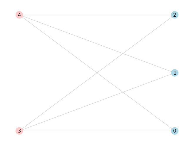
In this example, we demonstrate how MaxCut can be solved with Quantum Imaginary-Time Evolution. A detailed introduction to solving MaxCut with Quantum Approximate Optimization Algorithm can be found in this tutorial.

We start by defining the problem instance.

from qrisp import QuantumVariable, h, rzz
import networkx as nx

G = nx.Graph()
G.add_edges_from([[0,3],[0,4],[1,3],[1,4],[2,3],[2,4]])
N = G.number_of_nodes()

Next, we define the functions U_0 and exp_H for the QITE algorithm, and the classical cost function (similar to the tutorial):

def U_0(qv):
    h(qv)

def exp_H(qv, gamma):
    for pair in list(G.edges()):
        rzz(2*gamma, qv[pair[0]], qv[pair[1]])

def maxcut_obj(x):
    cut = 0
    for i, j in G.edges():
        if x[i] != x[j]:
            cut -= 1
    return cut

def maxcut_cost(meas_res):
    energy = 0
    for meas, p in meas_res.items():
        obj_for_meas = maxcut_obj(meas)
        energy += obj_for_meas * p
    return energy

With all the necessary ingredients, we use QITE to find an approximate solution to the MaxCut problem instance. At each iteration k, the optimal evolution time s_k is found by selecting the time that corresponds to the minimal value of the classical cost function maxcut_cost for a list of evolution times s_values = np.linspace(.01,.3,10). This could also be replaced by employing a more sophisticated optimization loop.

import numpy as np
import sympy as sp
from qrisp.qite import QITE

steps = 4
s_values = np.linspace(.01,.3,10)

theta = sp.Symbol('theta')
optimal_s = [theta]

# Caculate energy for initial state
qv = QuantumVariable(N)
U_0(qv)
E_0 = maxcut_cost(qv.get_measurement())

optimal_energies = [E_0]

for k in range(1,steps+1):

    # Perform k steps of QITE
    qv = QuantumVariable(N)
    QITE(qv, U_0, exp_H, optimal_s, k)
    qc = qv.qs.compile()

    # Find optimal evolution time
    # Use "precompliled_qc" keyword argument to avoid repeated compilation of the QITE circuit
    energies = [maxcut_cost(qv.get_measurement(subs_dic={theta:s_},precompiled_qc=qc)) for s_ in s_values]
    index = np.argmin(energies)
    s_min = s_values[index]

    optimal_s.insert(-1,s_min)
    optimal_energies.append(energies[index])

print(optimal_energies)

In the following, we print the 5 most likely solutions (for the optimal evolution times) together with their cost values.

qv = QuantumVariable(N)
QITE(qv, U_0, exp_H, optimal_s, steps)
results = qv.get_measurement()

print("5 most likely solutions")
max_five = sorted(results.items(), key=lambda item: item[1], reverse=True)[:5]
for res, prob in max_five:
    print(res, prob, maxcut_cost({res : 1}))

Finally, we visualize the most likely solution.

most_likely = max_five[0][0]
nx.draw(G, with_labels = True,
        node_color=['#FFCCCB' if most_likely[node]=='0' else '#ADD8E6' for node in G.nodes()],
        edge_color='#D3D3D3',
        pos = nx.bipartite_layout(G, [node for node in G.nodes() if most_likely[node]=='0']))