qrisp.app_phase_polynomial#
- app_phase_polynomial(*args, permeability='args', is_qfree=True, verify=False, **kwargs)#
Applies a phase function specified by a polynomial acting on a list of QuantumFloats. That is, this method implements the transformation
\[\ket{y_1}\dotsb\ket{y_n}\rightarrow e^{itP(y_1,\dotsc,y_n)}\ket{y_1}\dotsb\ket{y_n}\]where \(\ket{y_1},\dotsc,\ket{y_n}\) are QuantumFloats and \(P(y_1,\dotsc,y_n)\) is a polynomial in variables \(y_1,\dotsc,y_n\).
- Parameters:
- qf_listlist[QuantumFloat] or QuantumArray[QuantumFloat]
The list of QuantumFloats to evaluate the polynomial on.
- polySymPy expression
The polynomial to evaluate.
- symbol_listlist, optional
An ordered list of SymPy symbols associated to the QuantumFloats of
qf_list. By default, the symbols of the polynomial will be ordered alphabetically and then matched to the order inqf_list.- tFloat or SymPy expression, optional
The argument
tin the expression \(\exp(itP)\). The default is 1.
- Raises:
- Exception
Provided QuantumFloat list does not include the appropriate amount of elements to encode given polynomial.
Examples
We apply the phase function specified by the polynomial \(P(x,y) = \pi x + \pi xy\) on two QuantumFloats:
import sympy as sp
import numpy as np
from qrisp import QuantumFloat, h, app_phase_polynomial

x, y = sp.symbols('x y')
P = np.pi*x + np.pi*x*y

qf1 = QuantumFloat(3, signed = False)
qf2 = QuantumFloat(3,-1, signed = False)
h(qf1[0])
qf2[:]=0.5

app_phase_polynomial([qf1,qf2], P)
We print the
statevector:>>> print(qf1.qs.statevector()) sqrt(2)*(|0>*|0.5> - I*|1>*|0.5>)/2
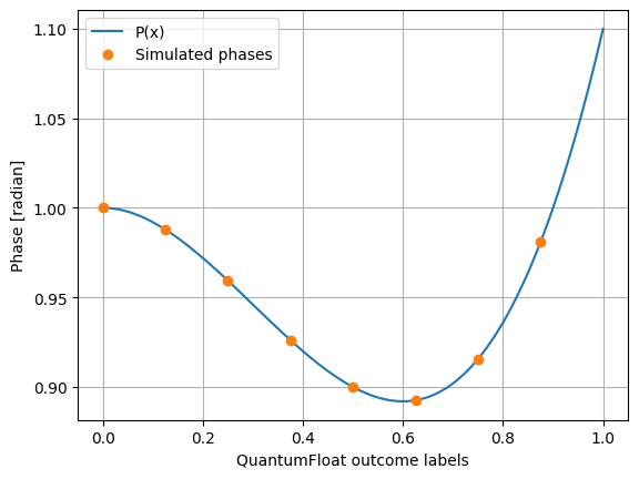
We apply the phase function specified by the polynomial \(P(x) = 1 - 0.9x^2 + x^3\) on a QuantumFloat:
import numpy as np
import sympy as sp
import matplotlib.pyplot as plt
from qrisp import QuantumFloat, h, app_phase_polynomial

x = sp.symbols('x')
P = 1-0.9*x**2+x**3

qf = QuantumFloat(3,-3)
h(qf)

app_phase_polynomial([qf],P)
To visualize the results we retrieve the
statevectoras a function and determine the phase of each entry.sv_function = qf.qs.statevector("function")
This function receives a dictionary of QuantumVariables specifiying the desired label constellation and returns its complex amplitude. We calculate the phases corresponding to the complex amplitudes, and compare the results with the values of the function \(P(x)\).
qf_values = np.array([qf.decoder(i) for i in range(2 ** qf.size)])
sv_phase_array = np.angle([sv_function({qf : i}) for i in qf_values])

P_func = sp.lambdify(x, P, 'numpy')
x_values = np.linspace(0, 1, 100)
y_values = P_func(x_values)
Finally, we plot the results.
plt.plot(x_values, y_values, label = "P(x)")
plt.plot(qf_values , sv_phase_array%(2*np.pi), "o", label = "Simulated phases")
plt.ylabel("Phase [radian]")
plt.xlabel("QuantumFloat outcome labels")
plt.grid()
plt.legend()
plt.show()